I am trying to construct a consensus WGCNA network from RNAseq data on three brain regions in two lines of zebrafish. My main hitch is with different outputs for the individual networks. I have constructed the consensus network using blockwiseConsensusModules (as shown in the code below) and saved the individual TOMs to disk. I then constructed individual networks for each brain region (one example is shown below) from each of the individual TOMs.

However, when I construct the individual networks from blockwiseModules using the same settings as before, I get a different network. I am thinking that something I am doing after TOM calculation in the first part is to blame, but I can't figure out what. The tutorial pages for this have been taken down so it's difficult for me to reference what is going on. My rationale for using the individual TOMs from blockwiseConsensusModules is that I figure that way the consensus network matches the dynamics in the individual networks as closely as possible, but the differences in these code outputs is making me think otherwise.

Can I relate the individual networks calculated with blockwiseModules to the consensus network? What is going on? Any help would be so appreciated.

net_cons <- blockwiseConsensusModules(multiExpr, TOMType = "signed", networkType = "signed", power = softPower, minModuleSize = 30, deepSplit = 2, pamRespectsDendro = FALSE, mergeCutHeight = 0.25, numericLabels = TRUE, verbose = 5, maxBlockSize = 25000, corType = "bicor", minKMEtoStay = 0)
save(net_cons, file = "net_cons.RData")

#consensus modules
table(net_cons$colors)
length(table(net_cons$colors))

#Bringing in calculated TOMS

load("individualTOM-Set1-Block1.RData")
tomDS_Dm <- tomDS
head(tomDS_Dm)
dim(tomDS_Dm)

# We like large modules, so we set the minimum module size relatively high:
minModuleSize = 30

# Call the hierarchical clustering function
geneTreeDm = hclust(as.dist(1-tomDS_Dm), method = "average")
# Plot the resulting clustering tree (dendrogram)
sizeGrWindow(12,9)
plot(geneTreeDm, xlab="", sub="", main = "Dm Gene clustering on TOM-based dissimilarity",
labels = FALSE, hang = 0.04)

# Module identification using dynamic tree cut:
dynamicModsDm = cutreeDynamic(dendro = geneTreeDm, distM = as.matrix(1-tomDS_Dm),
deepSplit = 2, pamRespectsDendro = FALSE,
minClusterSize = minModuleSize)
table(dynamicModsDm)

# Convert numeric labels into colors
dynamicColorsDm = labels2colors(dynamicModsDm)
table(dynamicColorsDm)
# Plot the dendrogram and colors underneath
sizeGrWindow(8,6)
plotDendroAndColors(geneTreeDm, dynamicColorsDm, "Dynamic Tree Cut",
dendroLabels = FALSE, hang = 0.03,
addGuide = TRUE, guideHang = 0.05,
main = "Gene dendrogram and module colors Dm")

# Calculate eigengenes
MEListDm = moduleEigengenes(as.data.frame(multiExpr[[1]]), colors = dynamicColorsDm)
MEsDm = MEListDm$eigengenes
# Calculate dissimilarity of module eigengenes
MEDissDm= 1-cor(MEsDm);
# Cluster module eigengenes
METreeDm = hclust(as.dist(MEDissDm), method = "average");
# Plot the result
sizeGrWindow(7, 6)
plot(METreeDm, main = "Clustering of module eigengenes Dm",
xlab = "", sub = "")

MEDissThres = 0.25
# Plot the cut line into the dendrogram
abline(h=MEDissThres, col = "red")
# Call an automatic merging function
mergeDm = mergeCloseModules(as.data.frame(multiExpr[[1]]), dynamicColorsDm, cutHeight = MEDissThres, verbose = 3)
# The merged module colors
mergedColorsDm = mergeDm$colors;
# Eigengenes of the new merged modules
mergedMEsDm = mergeDm$newMEs

sizeGrWindow(12, 9)
pdf(file = "geneDendro-3_Dm.pdf", wi = 9, he = 6)
plotDendroAndColors(geneTreeDm, cbind(dynamicColorsDm, mergedColorsDm),
c("Dynamic Tree Cut", "Merged dynamic"),
dendroLabels = FALSE, hang = 0.03,
addGuide = TRUE, guideHang = 0.05)
dev.off()
table(mergedColorsDm)

# Rename to moduleColors
moduleColorsDm = mergedColorsDm
# Construct numerical labels corresponding to the colors
colorOrder = c("grey", standardColors(50));
moduleLabelsDm = match(moduleColorsDm, colorOrder)-1;
MEsDm = mergedMEsDm
length(table(moduleColorsDm)) #51
table(moduleColorsDm)
sum(table(moduleLabelsDm))

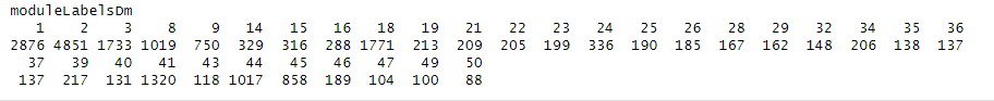
This is the module output I get from this approach:

net_Dm <- blockwiseModules(multiExpr[[1]]$data, TOMType = "signed", networkType = "signed", power = softPower, minModuleSize = 30, deepSplit = 2, pamRespectsDendro = FALSE, mergeCutHeight = 0.25, numericLabels = TRUE, verbose = 5, maxBlockSize = 25000, corType = "bicor", minKMEtoStay = 0)
save(net_Dm, file = "net_Dm.RData")
table(net_Dm$colors)

This is the output I get from this approach:

Session Info below:

R version 4.3.0 (2023-04-21 ucrt) Platform: x86_64-w64-mingw32/x64 (64-bit) Running under: Windows 10 x64 (build 19045)

Matrix products: default

locale: 1 LC_COLLATE=English_United States.utf8 LC_CTYPE=English_United States.utf8 LC_MONETARY=English_United States.utf8 [4] LC_NUMERIC=C LC_TIME=English_United States.utf8

time zone: America/Chicago tzcode source: internal

attached base packages: 1 stats graphics grDevices utils datasets methods base

other attached packages: 1 lubridate_1.9.2 forcats_1.0.0 stringr_1.5.0 dplyr_1.1.2 purrr_1.0.1
[6] readr_2.1.4 tidyr_1.3.0 tibble_3.2.1 ggplot2_3.4.2 tidyverse_2.0.0
[11] WGCNA_1.72-1 fastcluster_1.2.3 dynamicTreeCut_1.63-1

loaded via a namespace (and not attached): 1 tidyselect_1.2.0 blob_1.2.4 Biostrings_2.68.1 bitops_1.0-7
[5] fastmap_1.1.1 RCurl_1.98-1.12 digest_0.6.31 rpart_4.1.19
[9] timechange_0.2.0 lifecycle_1.0.3 cluster_2.1.4 survival_3.5-5
[13] KEGGREST_1.40.0 RSQLite_2.3.1 magrittr_2.0.3 compiler_4.3.0
[17] rlang_1.1.1 Hmisc_5.1-0 tools_4.3.0 utf8_1.2.3
[21] yaml_2.3.7 data.table_1.14.8 knitr_1.43 htmlwidgets_1.6.2
[25] bit_4.0.5 withr_2.5.0 foreign_0.8-84 BiocGenerics_0.46.0
[29] nnet_7.3-19 grid_4.3.0 stats4_4.3.0 preprocessCore_1.62.1
[33] fansi_1.0.4 colorspace_2.1-0 GO.db_3.17.0 scales_1.2.1
[37] iterators_1.0.14 cli_3.6.1 rmarkdown_2.22 crayon_1.5.2
[41] generics_0.1.3 rstudioapi_0.14 tzdb_0.4.0 httr_1.4.6
[45] DBI_1.1.3 cachem_1.0.8 zlibbioc_1.46.0 splines_4.3.0
[49] parallel_4.3.0 impute_1.74.1 AnnotationDbi_1.62.1 XVector_0.40.0
[53] matrixStats_0.63.0 base64enc_0.1-3 vctrs_0.6.2 Matrix_1.5-4.1
[57] hms_1.1.3 IRanges_2.34.0 S4Vectors_0.38.1 bit64_4.0.5
[61] Formula_1.2-5 htmlTable_2.4.1 foreach_1.5.2 glue_1.6.2
[65] codetools_0.2-19 stringi_1.7.12 gtable_0.3.3 GenomeInfoDb_1.36.0
[69] munsell_0.5.0 pillar_1.9.0 htmltools_0.5.5 GenomeInfoDbData_1.2.10 [73] R6_2.5.1 doParallel_1.0.17 evaluate_0.21 lattice_0.21-8
[77] Biobase_2.60.0 png_0.1-8 backports_1.4.1 memoise_2.0.1
[81] Rcpp_1.0.10 gridExtra_2.3 checkmate_2.2.0 xfun_0.39
[85] pkgconfig_2.0.3