
Hello!
I am having a blast getting acquainted with the EBImage package and generating an R script to analyze x-ray images of seed. We have about 150 x-ray images that are 5888 x 4620 pixels. Within the image, there are two "reference disks" we 3D printed and they are 18.8mm in diameter. Between those disks are 2 rows of 5 seeds. We are trying to identify the length, width, and area of each hull and kernel. That way, we can directly identify the kernel/hull ratio for breeding purposes.
The main concerns I have are:
- Is creating a binary image with "fillHull(greyImage > 0.20" and then performing morphological opening with "opening(binaryImage, makeBrush(15, shape='disc'))" a reasonable or appropriate approach? I know this package has many options and these seemed like the best options (Introduction to EBImage)
- If I do stick with these two key operations, is there any opinions on how exactly I should determine the values (e.g. 0.20 for fillHull and 15 for makeBrush)? For some images, 0.15 is sufficient, but for others I need 0.22 or higher with fillHull. As for makeBrush, I picked 15 because it seems like a decent balance of appropriate smoothing of edges without excess.
- Would it make sense to create a code loop that uses shapeStats' s.area and the number of rows/identified objects to adjust the fillHull parameter until all objects are greater than a "safe minimum" s.area? Or perhaps just loop until 10 objects of similar size are detected in addition to the two reference disks (maybe start at fillHull > 0.10, incrementing by 0.01 each loop)? I was thinking of doing this but I have concerns that the measurements wouldn't be consistent enough. As a result I have been leaning toward just using a relatively high value between 0.20 and 0.25.
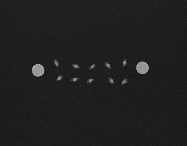
Here is an example image I generated using this package. You can see the 2 reference disks, 10 seeds, and lengths and widths lines drawn on the original x-ray image, calculated using the EBImage package.
Here is the most relevant code chunk:
# Convert to grayscale
greyImage <- channel(img, "gray")

# Make binary image with set threshold
binaryImage <- fillHull(greyImage > 0.20)

# Perform morphological opening to remove small noise elements
openedImage <- opening(binaryImage, makeBrush(15, shape='disc'))
Thank you for your time! Here is my sessionInfo:
sessionInfo( )
R version 4.3.0 (2023-04-21)
Platform: x86_64-pc-linux-gnu (64-bit)
Running under: Ubuntu 22.04.3 LTS

Matrix products: default
BLAS:   /usr/lib/x86_64-linux-gnu/openblas-pthread/libblas.so.3
LAPACK: /usr/lib/x86_64-linux-gnu/openblas-pthread/libopenblasp-r0.3.20.so;  LAPACK version 3.10.0

locale:
 [1] LC_CTYPE=en_US.UTF-8       LC_NUMERIC=C               LC_TIME=en_US.UTF-8        LC_COLLATE=en_US.UTF-8     LC_MONETARY=en_US.UTF-8    LC_MESSAGES=en_US.UTF-8
 [7] LC_PAPER=en_US.UTF-8       LC_NAME=C                  LC_ADDRESS=C               LC_TELEPHONE=C             LC_MEASUREMENT=en_US.UTF-8 LC_IDENTIFICATION=C

time zone: Etc/UTC
tzcode source: system (glibc)

attached base packages:
[1] stats     graphics  grDevices utils     datasets  methods   base

other attached packages:
[1] EBImage_4.42.0

loaded via a namespace (and not attached):
 [1] digest_0.6.31       fastmap_1.1.1       lattice_0.21-8      abind_1.4-5         jpeg_0.1-10         BiocGenerics_0.46.0 RCurl_1.98-1.12     htmltools_0.5.5
 [9] png_0.1-8           bitops_1.0-7        fftwtools_0.9-11    cli_3.6.1           grid_4.3.0          compiler_4.3.0      rstudioapi_0.14     tools_4.3.0
[17] ellipsis_0.3.2      yaml_2.3.7          tiff_0.1-11         locfit_1.5-9.8      jsonlite_1.8.5      htmlwidgets_1.6.2   rlang_1.1.1
And if relevant, here is my full script that was used to generate the image I shared:
# Load test image as "img"
img <- readImage("~/SilphiumXrayAnalysis/5-43-35_4_I20220214155857.tif")

# Define the step size for iterating over the seed's length
# A smaller step size increases accuracy but takes longer to compute
# 1 would be checking width at every pixel, which could be around 300
# A larger step size decreases accuracy but speeds up computation.
# You may adjust this depending on the required precision and computational resources.
stepSize <- 25  # Adjust this as needed

# Convert to grayscale
greyImage <- channel(img, "gray")

# Make binary image with set threshold
binaryImage <- fillHull(greyImage > 0.20)

# Perform morphological opening to remove small noise elements
openedImage <- opening(binaryImage, makeBrush(15, shape='disc'))

# Label the connected components in the opened image
labeledImage <- bwlabel(openedImage)

# Display processed image
display(labeledImage)

# Calculate shape statistics
shapeStats <- computeFeatures.shape(labeledImage)

# Sort shapeStats by area (two biggest are reference disks)
shapeStats <- shapeStats[order(shapeStats[,"s.area"], decreasing = TRUE),]

# Calculate the centroids and features of the objects in the labeled image
momentStats <- computeFeatures.moment(labeledImage)

# Sort momentStats by majoraxis (two biggest are reference disks)
momentStats <- momentStats[order(momentStats[,"m.majoraxis"], decreasing = TRUE),]

# Assuming the first two rows in shapeStats are the reference disks, we exclude them
shapeStatsSeeds <- shapeStats[-c(1,2),]
momentStatsSeeds <- momentStats[-c(1,2),]

# Calculate the average radius in pixels of the two reference disks
refDiskRadiusPixels1 <- shapeStats[1, "s.radius.max"]
refDiskRadiusPixels2 <- shapeStats[2, "s.radius.max"]
avgRefDiskRadiusPixels <- mean(c(refDiskRadiusPixels1, refDiskRadiusPixels2))

# Calculate the pixel-to-mm conversion ratio for lines
pixelToMmRatio <- 18.8 / (avgRefDiskRadiusPixels * 2)

# Calculate the conversion factor for area (square of pixelToMmRatio)
areaConversionFactor <- pixelToMmRatio^2

# The maximum length of each seed is twice the maximum radius
seedLengthsPixels <- shapeStatsSeeds[,"s.radius.max"] * 2

# Apply the line ratio to convert the seed lengths to mm
seedLengthsMm <- seedLengthsPixels * pixelToMmRatio

#Store the area in pixels of each seed
seedAreasPixels <- shapeStatsSeeds[,"s.area"]

# Apply the area ratio to convert the seed areas to mm^2
seedAreasMm2 <- seedAreasPixels * areaConversionFactor

# Additional variables to store width line endpoints
widthLineStartX <- widthLineStartY <- widthLineEndX <- widthLineEndY <- numeric(nrow(momentStatsSeeds))

# Calculate width for each seed
seedWidthsPixels <- numeric(nrow(momentStatsSeeds))
for (i in 1:nrow(momentStatsSeeds)) {
  centerX <- momentStatsSeeds[i, "m.cx"]
  centerY <- momentStatsSeeds[i, "m.cy"]
  lengthAngle <- momentStatsSeeds[i, "m.theta"]
  widthAngle <- lengthAngle + pi / 2
  maxDistAlongLength <- shapeStatsSeeds[i, "s.radius.max"]
  maxWidth <- 0

  for (dist in seq(-maxDistAlongLength, maxDistAlongLength, by = stepSize)) {
    lengthX <- centerX + cos(lengthAngle) * dist
    lengthY <- centerY + sin(lengthAngle) * dist
    startX <- lengthX
    startY <- lengthY
    endX <- startX
    endY <- startY
    currentWidth <- 0

    while (endX >= 1 && endX <= ncol(labeledImage) && endY >= 1 && endY <= nrow(labeledImage) && labeledImage[round(endX), round(endY)] != 0) {
      endX <- endX + cos(widthAngle)
      endY <- endY + sin(widthAngle)
      currentWidth <- sqrt((startX - endX)^2 + (startY - endY)^2)
    }

    while (startX >= 1 && startX <= ncol(labeledImage) && startY >= 1 && startY <= nrow(labeledImage) && labeledImage[round(startX), round(startY)] != 0) {
      startX <- startX - cos(widthAngle)
      startY <- startY - sin(widthAngle)
      currentWidth <- sqrt((startX - endX)^2 + (startY - endY)^2)
    }

    if (currentWidth > maxWidth) {
      maxWidth <- currentWidth
      widthLineStartX[i] <- startX
      widthLineStartY[i] <- startY
      widthLineEndX[i] <- endX
      widthLineEndY[i] <- endY
    }
  }

  seedWidthsPixels[i] <- maxWidth
}

# Apply the line ratio to convert the seed widths to mm
seedWidthsMm <- seedWidthsPixels * pixelToMmRatio

# Combine the lengths and widths into a data frame
seedSizesMm <- data.frame(
  Length_mm = seedLengthsMm,
  Width_mm = seedWidthsMm,
  Area_mm2 = seedAreasMm2
)

# Display the length and width in mm for each seed
print(seedSizesMm)

# Drawing the lines on the original image
plot(img)
for (i in 1:nrow(momentStatsSeeds)) {
  # Draw length line
  lengthHalf <- shapeStatsSeeds[i, "s.radius.max"]
  lengthAngle <- momentStatsSeeds[i, "m.theta"]
  segments(momentStatsSeeds[i, "m.cx"] - cos(lengthAngle) * lengthHalf,
           momentStatsSeeds[i, "m.cy"] - sin(lengthAngle) * lengthHalf,
           momentStatsSeeds[i, "m.cx"] + cos(lengthAngle) * lengthHalf,
           momentStatsSeeds[i, "m.cy"] + sin(lengthAngle) * lengthHalf,
           col = "#DC2DAB")

  # Draw width line
  segments(widthLineStartX[i], widthLineStartY[i], widthLineEndX[i], widthLineEndY[i], col = "#F3844A")
}
Only thing I realized that I should change is the use of m.majoraxis from computeFeatures.moment instead of s.radius.max from computeFeatures.shape. Using m.majoraxis from computeFeatures.moment provides a more accurate measurement of the actual length for elongated or irregularly shaped seeds, as it represents the longest line that can be drawn across the object. In contrast, using s.radius.max from computeFeatures.shape and doubling it for length could lead to overestimations, especially for non-circular seeds, since the maximum radius might not reflect the typical width of the seed.
Dear Brian
There are certainly several ways to approach this. You have quite a lot of prior information (number of seeds, expected seed size range and shape) and it's good to use these in the algorithm, either for parameter adaptation or for quality control.
As for the binarization threshold, you could try to estimate it from the histogram: e.g., 90% quantile + 0.1. This assumes that more than 90% of the pixels are background, and that foreground intensities are more than 0.1 intensity units brighter. You can also work on the original intensity scale if that is more intuitive or more robust.
As you suggest, you can fill holes using fillHull and smooth the borders using morpholgical opening, but I am not even sure it is that important.
My main suggestion that deviates from your approach would be to use robust estimator of mean and covariance matrix on the thus obtained pixel sets (i.e. their x and y coordinates). The square roots of the eigenvalues of the covariance would immediately give you length and width. (see e.g. https://search.r-project.org/CRAN/refmans/robust/html/covRob.html)
There is also nothing wrong with your approach afaIcs, just maybe a bit more complicated than necessary.