I want to know which methods are commonly used for RNA seq data if the goal is to identify monotonic increasing or decreasing gene expression over time or across stages using the results of differential gene expression analysis?
The easiest way is to fit a time trend, select genes with a significant F-test and then check whether the fitted values are in monotonic order.
I tried to fit a time trend model for each gene but it takes forever. It seems like it is computationally expensive. Can I fit the linear model for all genes simultaneously using a matrix?
Processor: 11th Gen Intel(R) Core(TM) i7-1165G7 @ 2.80GHz 2.80 GHz RAM:16.0 GB
  time_trend_model <- lapply(names(ordered_counts)[1:5429], function(gene) {
  formula <- as.formula(paste(ordered_counts, "~ stage"))
  lm(formula, data = ordered_counts)
  })
Fitting genewise time trends take only a few seconds using either limma or edgeR, even for a large dataset and even on a laptop computer. Both packages perform F-tests. There are examples in the limma and edgeR User's guides, but it is just a standard analysis for either of those packages.
I was certainly not recommending that you fit linear models directly to ordered counts. That wouldn't make any sense statistically, even it was computationally efficient.
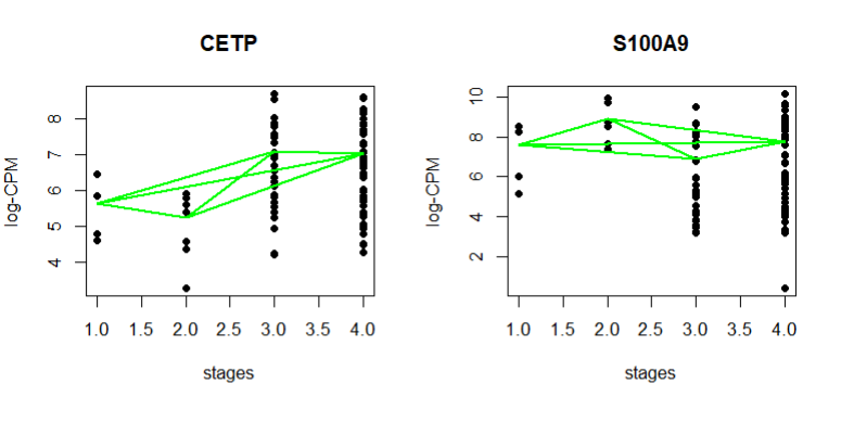
I am not sure why the plots are different from the user guide. I am dealing with defined stages while the user guide deals with hours
design = model.matrix(~0 + dge_stage$samples$Stage)
colnames(design)[1]="Stage1"
colnames(design)[2]="Stage2"
colnames(design)[3]="Stage3"
colnames(design)[4]="Stage4"

stages=as.numeric(c(dge_stage$samples$Stage))

polycurve = poly(stages, degree=3)
design <- model.matrix(~ polycurve)

dge_stage <- estimateGLMCommonDisp(dge_stage, design)

dge_stage <- estimateGLMTagwiseDisp(dge_stage, design)

glmfit=glmQLFit(dge_stage, design=design)
plotQLDisp(glmfit)

Time_FTest=glmQLFTest(glmfit, coef=ncol(glmfit$design))

#The topTags function lists the top set of genes with most
#significant time effects.

tab <- as.data.frame(topTags(Time_FTest, n=30))

summary(decideTests(Time_FTest))

logCPM.obs <- cpm(dge_stage$counts, log=TRUE, prior.count=Time_FTest$prior.count)
logCPM.fit <- cpm(Time_FTest, log=TRUE)


par(mfrow=c(2,2))
for(i in 1:10) {
GeneID <- row.names(tab)[i]
Symbol <- tab$hgnc_symbol[i]
logCPM.obs.i <- logCPM.obs[GeneID,]
logCPM.fit.i <- logCPM.fit[GeneID,]
plot(stages, logCPM.obs.i, ylab="log-CPM", main=Symbol, pch=16)
lines(stages, logCPM.fit.i, col="green", lwd=2)
}

Also, results of summary(decideTests(Time_FTest))

polycurve3
Down            0
NotSig       5429
Up                0
Use of this site constitutes acceptance of our User Agreement and Privacy Policy.


Cross-posted to Biostars https://www.biostars.org/p/9585490/