I have a 10x 5' scRNA-seq dataset where Cell Ranger (v9.0.0) reports 64,610 non-empty droplets. This is plausible since it comes from an hashtagged and superloaded GEM-X capture.

I always run DropletUtils::emptyDrops() by way of comparison, and here got very different results: 27,739 non-empty droplets. Knowing that the default value of the alpha = Inf parameter changed recently-ish, I repeated this with the former default alpha = NULL and recovered numbers comparable to Cell Ranger: 72,162 non-empty droplets. I'm trying to understand which approach to put more weight on, and conducted some experiments (copied below). I can share the count matrix, (x; ~300 MB) if it would be helpful. Any suggestions and explanations appreciated.

Thanks, Pete

library(DropletUtils)

x <- readRDS("x.rds")

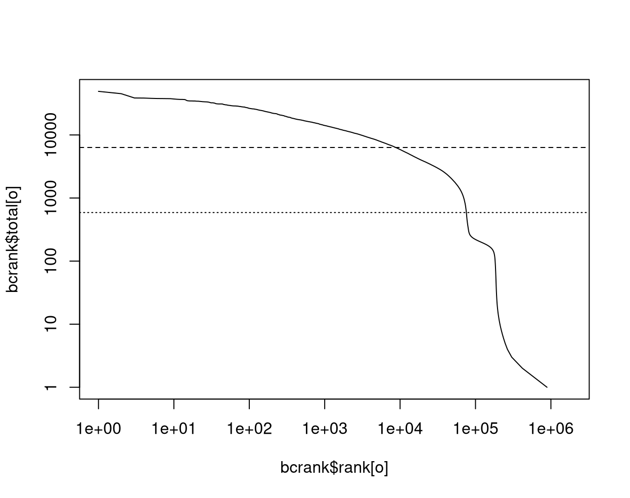
bcrank <- barcodeRanks(x)
uniq <- !duplicated(bcrank$rank)
plot(
  bcrank$rank[uniq],
  bcrank$total[uniq],
  log = "xy",
  xlab = "Rank",
  ylab = "Total UMI count",
  cex.lab = 1.2)
#> Warning in xy.coords(x, y, xlabel, ylabel, log): 1 y value <= 0 omitted from
#> logarithmic plot
abline(h = metadata(bcrank)$inflection, col = "darkgreen", lty = 2)
abline(h = metadata(bcrank)$knee, col = "dodgerblue", lty = 2)
legend(
  "bottomleft",
  legend = c("Inflection", "Knee"),
  col = c("darkgreen", "dodgerblue"),
  lty = 2,
  cex = 1.2)

# emptyDrops under default settings --------------------------------------------

lower <- 100
set.seed(666)
ed_alpha_inf <- emptyDrops(x, lower = lower, test.ambient = TRUE)
ed_alpha_null <- emptyDrops(x, lower = lower, test.ambient = TRUE, alpha = NULL)

sum(ed_alpha_inf$FDR <= 0.001, na.rm = TRUE)
#> [1] 27739
sum(ed_alpha_null$FDR <= 0.001, na.rm = TRUE)
#> [1] 72162

par(mfrow = c(1, 2))
hist(
  ed_alpha_inf$PValue[ed_alpha_inf$Total <= lower & ed_alpha_inf$Total > 0],
  xlab = "P-value",
  main = "alpha = Inf",
  col = "grey80")
hist(
  ed_alpha_null$PValue[ed_alpha_null$Total <= lower & ed_alpha_null$Total > 0],
  xlab = "P-value",
  main = "alpha = NULL",
  col = "grey80")

# emptyDrops under expectation of ~60,000 non-empty droplets -------------------

by.rank <- 70000
set.seed(666)
ed_alpha_inf <- emptyDrops(x, by.rank = by.rank, test.ambient = TRUE)
ed_alpha_null <- emptyDrops(x, by.rank = by.rank, test.ambient = TRUE, alpha = NULL)
sum(ed_alpha_inf$FDR <= 0.001, na.rm = TRUE)
#> [1] 30369
sum(ed_alpha_null$FDR <= 0.001, na.rm = TRUE)
#> [1] 49461

# NOTE: Extract lower (doesn't depend on alpha)
lower <- metadata(ed_alpha_inf)$lower
lower
#> [1] 992
par(mfrow = c(1, 2))
hist(
  ed_alpha_inf$PValue[
    ed_alpha_inf$Total <= lower & ed_alpha_inf$Total > 0],
  xlab = "P-value",
  main = "alpha = Inf",
  col = "grey80")
hist(
  ed_alpha_null$PValue[
    ed_alpha_null$Total <= lower & ed_alpha_null$Total > 0],
  xlab = "P-value",
  main = "alpha = NULL",
  col = "grey80")

# More extreme version of the above --------------------------------------------

by.rank <- 100000
set.seed(666)
ed_alpha_inf <- emptyDrops(x, by.rank = by.rank, test.ambient = TRUE)
ed_alpha_null <- emptyDrops(x, by.rank = by.rank, test.ambient = TRUE, alpha = NULL)
sum(ed_alpha_inf$FDR <= 0.001, na.rm = TRUE)
#> [1] 36717
sum(ed_alpha_null$FDR <= 0.001, na.rm = TRUE)
#> [1] 65752

# NOTE: Extract lower (doesn't depend on alpha)
lower <- metadata(ed_alpha_inf)$lower
lower
#> [1] 220
par(mfrow = c(1, 2))
hist(
  ed_alpha_inf$PValue[
    ed_alpha_inf$Total <= lower & ed_alpha_inf$Total > 0],
  xlab = "P-value",
  main = "alpha = Inf",
  col = "grey80")
hist(
  ed_alpha_null$PValue[
    ed_alpha_null$Total <= lower & ed_alpha_null$Total > 0],
  xlab = "P-value",
  main = "alpha = NULL",
  col = "grey80")

# emptyDropsCellRanger() -------------------------------------------------------

# NOTE: Unsure how closely this actually mimics what Cell Ranger is doing, but
#       including because it's easy enough to do.
ed_cr <- emptyDropsCellRanger(x, n.expected.cells = 60000)
sum(ed_cr$FDR <= 0.001, na.rm = TRUE)
#> [1] 63190

I suspect the real problem is that the knee point is not being identified correctly in your plot. Visually, I would put the knee point somewhere at the midpoint between the blue and green lines, which should give you something along the lines of "must keep 50000 cells", though it's hard to say with the log scale.

To recap, emptyDrops() will keep all droplets above the knee point, to ensure that high-coverage droplets are retained even if they look similar to the ambient solution. This is designed to maintain detection power even for homogeneous cell populations where the ambient solution might be just a copy of the population (and thus the null hypothesis would never be rejected by the multinomial model).

Unfortunately, knee point detection is somewhat heuristic. There is a proper way to do it based on maximizing the curvature, but it depends on the second derivative and is unstable for empirically-fitted curves. So in https://github.com/MarioniLab/DropletUtils/pull/117, we switched to a much simpler algorithm whereby we draw a line from the 50th cell (see exclude.from= in barcodeRanks()) to the inflection point, and set the knee point to the location on the curve that maximizes the vertical distance from the line.

This approach worked pretty well on most of my datasets (see the results in #117), but in your case, it doesn't quite pick the right location. I think this is because you have so many cells that the 50th cell is quite far away from the inflection point. This gives an opportunity for other local maxima to be considered, and in your case, the chosen location is quite far away from the visual knee point. I'd guess that this is still a knee point of some sort - one can see a bit of lump in the curve - but it's not the one that gives us most detected cells.

The change in alpha= just exposes the real problem. Previously, the anticonservativeness of alpha=NULL (see https://github.com/MarioniLab/DropletUtils/pull/118) was covering up the conservative choice of the knee point. Now that the p-values are properly sized, the consequences of the earlier knee point are more apparent.

The solution might be as simple as picking a better left-side point to define our line. One idea might be to take the x-coordinate of the inflection point, divide it by 10, and use that location on the curve to define our line to the inflection point. This restricts the knee point identification to the interval immediately preceding the inflection point, and ensures that the knee point identification doesn't get distracted by other maxima at lower x-coordinates. Probably something like the code below, see if it works for you:

library(DropletTestFiles)
path <- getTestFile("tenx-3.1.0-5k_pbmc_protein_v3/1.0.0/raw.h5")

library(DropletUtils)
se <- read10xCounts(path, type="HDF5")
mat <- as(assay(se), "SVT_SparseMatrix")

# Paraphrased from barcodeRanks.
totals <- colSums(mat)
o <- order(totals, decreasing=TRUE)
stuff <- rle(totals[o])
run.rank <- cumsum(stuff$lengths) - (stuff$lengths-1)/2
run.totals <- stuff$values
keep <- run.totals > 100 # i.e., lower=100
y <- log10(run.totals[keep])
x <- log10(run.rank[keep])

edge.out <- DropletUtils:::.find_curve_bounds(x=x, y=y, exclude.from=50)
left.edge <- edge.out["left"]
right.edge <- edge.out["right"]
inflection <- 10^(y[right.edge])

new.left.rank <- x[right.edge] - 1 # -1 as we're in log10 units already.
new.left.edge <- findInterval(new.left.rank, x)
new.keep <- new.left.edge:right.edge

curx <- x[new.keep]
cury <- y[new.keep]
xbounds <- curx[c(1L, length(new.keep))]
ybounds <- cury[c(1L, length(new.keep))]
gradient <- diff(ybounds)/diff(xbounds)
intercept <- ybounds[1] - xbounds[1] * gradient
above <- which(cury >= curx * gradient + intercept)
dist <- abs(gradient * curx[above] - cury[above] + intercept)/sqrt(gradient^2 + 1)
knee <- 10^(cury[above[which.max(dist)]])

o <- order(current$rank)
plot(current$rank[o], current$total[o], log="xy", type="l")
abline(h=knee, lty=2)
abline(h=infl, lty=3)

FWIW emptyDropsCellranger() defines its "must keep" threshold differently - namely, using the n.expected.cells and max.percentile arguments - so it doesn't suffer from the knee point problem.