
Hello,
My questions are about using ZINB-WaVE.
I have written out the main steps I took to reach this point. If you don't have the time to read it, my questions are written under the heading below. Thank you!
Questions
- How should I decide on a value for
Kwhen runningzinbwave()? Will this impact observational weights when using DESeq2?- I have so far tested
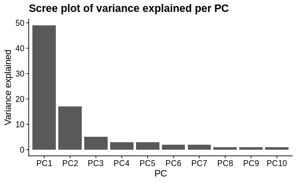
K=2andK=3, based on principal components analysis identifying 2 major sources of variation (shown below). There are 4 different biological conditions and 1 technical covariate, however, so shouldKbe set to reflect this?
- I have so far tested
Should I filter genes for the dimensionality reduction step?
- I have tested the top 1000 most variable genes and the entire set of 16000. If I use 16000 genes, I need a higher epsilon value (16000 instead of 1000) to achieve a similar looking representation.
- For calculating observational weights for DESeq2, I am guessing I will use my entire set of 16000 genes?
How should I decide on a value for epsilon?
- I have tested epsilon values of 1000, 16000, 1e6, 1e12. The impact of changing epsilon seems to depend heavily on the choice of
Kand the number of genes used.
- I have tested epsilon values of 1000, 16000, 1e6, 1e12. The impact of changing epsilon seems to depend heavily on the choice of
Introduction
I am working with a bulk RNA-Seq dataset in which I used translating ribosome affinity purification to extract ribosome-bound RNA from a specific cell type in different regions of mouse brain. The library was prepared using an ultra low input protocol, as I could reliably obtain ~100 pg per sample (in some regions, this cell type is very rare). Each sample was sequenced to a depth of ~25 million reads. There are 120 samples in total, collected over 8 batches (every biological condition was collected in each batch).
I suspect there may be zero inflation in the count values of all samples, as I try to demonstrate below.
Zero inflation: Calculating dropout rate
To check for zero-inflation, I did the following:
# dds is a DESeq2 object created from a salmon > tximeta > DESeq2 workflow

# filter genes with less than 5 counts in at least 10 samples
dds <- dds[rowSums(counts(dds) >= 5) >= 10,]

# check dimensions
dim(dds)
# ~16000 genes, 120 samples

## calculate dropout
# extract counts (as I could not set 0 values to NA in the DESeq object)
cts <- counts(dds)
# set 0 values to NA
cts[cts == 0] <- NA
# calculate per gene mean count (excluding zero counts) and the proportion of zeros
dropouts <- tibble(mean = rowMeans(cts, na.rm = T),
       dropouts = rowSums(is.na(cts))/ncol(cts))

# quantile of dropouts
quantile(dropouts$dropouts, seq(0.1, 1, 0.1))
#        10%         20%         30%         40%         50%         60%         70%
#0.008333333 0.075000000 0.183333333 0.300000000 0.416666667 0.533333333 0.650000000
#        80%         90%        100%
#0.750000000 0.841666667 0.916666667

# plot mean vs dropouts
dropouts %>%
  ggplot(aes(x = log10(mean),
             y = dropouts)) +
  geom_point(alpha = 0.1)
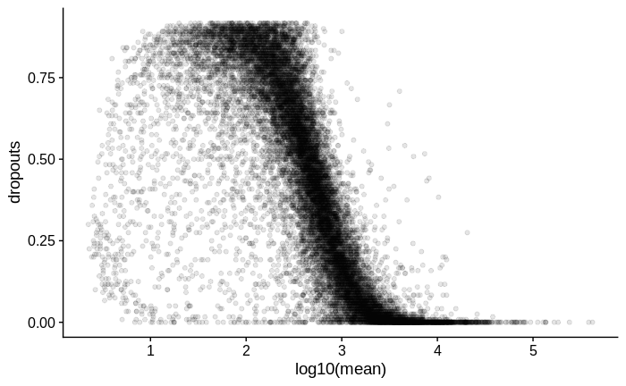
For comparison, below is the same plot for another dataset in which I used Smart-Seq2 with a larger input amount of RNA of the same type of samples:
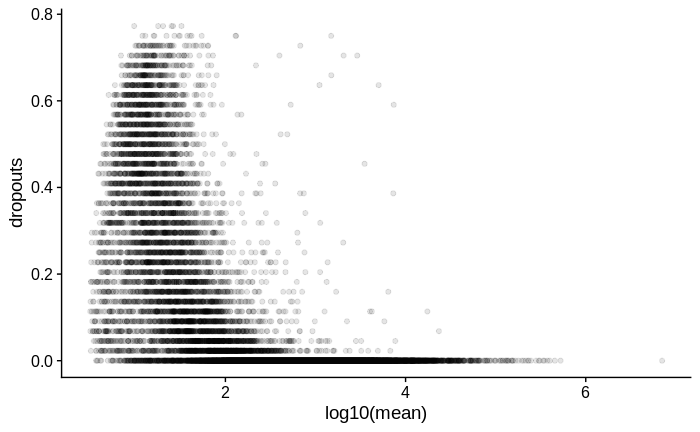
I then went on to look at the dispersion estimates.
Dispersion
# calculate size factors and dispersion
dds <- estimateSizeFactors(dds, "poscounts")
dds <- estimateDispersions(dds, fitType = "local")

# plot dispersion estimates
plotDispEsts(dds)
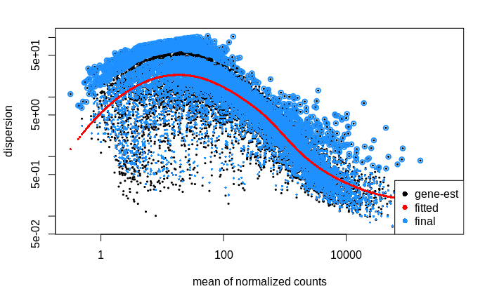
My interpretation of this plot is that the dispersion of lower count genes (<1000 counts) is large; large enough to weaken my ability to detect differentially expressed genes within this count range. Is this correct?
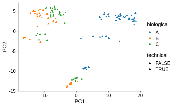
PCA
I performed principal components analysis to look at how the samples differ. I used the top 1000 most variable genes. I expected 1 major technical and 1 major biological sample covariate to cause separation and this was confirmed. There is a large drop in variance explained by subsequent PC's, although they may represent variation due to other biological conditions tested (not shown).
# subsetting 1000 most variable genes
vars <- counts(dds) %>% rowVars
names(vars) <- rownames(dds)
vars <- sort(vars, decreasing = TRUE)
zidds <- dds[names(vars)[1:1000],]

# recalculate size factors and dispersion - is this necessary?
zidds <- estimateSizeFactors(zidds, "poscounts")
zidds <- estimateDispersions(zidds, fitType = "local")

# variance stabilising transformation
vsd <- vst(zidds)

# make pea object
pca <- prcomp(t(assay(vsd)))
# add colData
pca$x <- pca$x %>%
      as_tibble(rownames = identifier) %>%
      inner_join(colData(zidds), copy = TRUE)

# plot PC1 vs PC2
pca$x %>%
  ggplot(aes(x = PC1,
             y = PC2,
             colour = biological,
             shape = technical)) +
  geom_point()
# calculate the variation per component
var_explained0 <- pca$sdev^2/sum(pca$sdev^2) #Calculate PC variance
names(var_explained0) <- colnames(pca$x)
var_explained <- as_tibble(var_explained0,
                            rownames = "PC") %>%
mutate(var = paste0((round(var_explained0*100)), ' %', sep = '')) %>%
select(PC, var)

pca$var_explained <- var_explained

# scree splot
pca$var_explained %>%
  slice_head(n=10) %>%
  mutate(PC = factor(PC, levels = c("PC1", "PC2", "PC3", "PC4", "PC5",
                                    "PC6", "PC7", "PC8", "PC9", "PC10")),
         var = as.integer(str_extract(var, pattern = "[:digit:]+"))) %>%
  ggplot(aes(x = PC,
             y = var)) +
  geom_col()
ZINB-WaVE
I have been following the ZINB-WaVE vignette and the deseq2-zinbwave workflow to try to account for zero inflation.
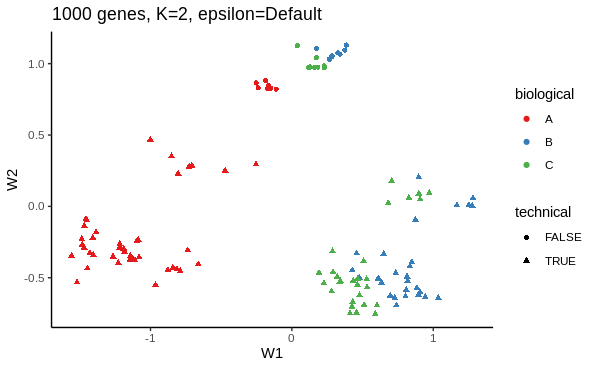
I first want to use ZINB-WaVE's dimensionality reduction method to see how adjusting for dropout influences the low dimension representation. Below is an example of my working.
# ZINB dimensionality reduction with 1000 most variable genes, K = 2, epsilon default

zinb <- zinbwave(zidds,
                K = 2)

W <- reducedDim(zinb)

as_tibble(W, rownames = "sample_name") %>%
  inner_join(colData(zinb), copy = TRUE) %>%
    ggplot(aes(W1,
                      W2,
                      colour=biological,
                      shape=technical)) +
    geom_point()
sessionInfo( )

R version 4.0.3 (2020-10-10)
Platform: x86_64-pc-linux-gnu (64-bit)
Running under: Ubuntu 18.04.5 LTS

Matrix products: default
BLAS:   /usr/lib/x86_64-linux-gnu/blas/libblas.so.3.7.1
LAPACK: /usr/lib/x86_64-linux-gnu/lapack/liblapack.so.3.7.1

locale:
 [1] LC_CTYPE=en_GB.UTF-8       LC_NUMERIC=C
 [3] LC_TIME=en_GB.UTF-8        LC_COLLATE=en_GB.UTF-8
 [5] LC_MONETARY=en_GB.UTF-8    LC_MESSAGES=en_GB.UTF-8
 [7] LC_PAPER=en_GB.UTF-8       LC_NAME=C
 [9] LC_ADDRESS=C               LC_TELEPHONE=C
[11] LC_MEASUREMENT=en_GB.UTF-8 LC_IDENTIFICATION=C

attached base packages:
 [1] parallel  stats4    grid      stats     graphics  grDevices datasets
 [8] utils     methods   base

other attached packages:
 [1] edgeR_3.32.1                limma_3.46.0
 [3] zinbwave_1.12.0             SingleCellExperiment_1.12.0
 [5] apeglm_1.12.0               biomaRt_2.46.1
 [7] BiocParallel_1.24.1         org.Mm.eg.db_3.12.0
 [9] GenomicFeatures_1.42.1      AnnotationDbi_1.52.0
[11] rhdf5_2.34.0                tximport_1.18.0
[13] DESeq2_1.30.0               SummarizedExperiment_1.20.0
[15] Biobase_2.50.0              MatrixGenerics_1.2.0
[17] matrixStats_0.57.0          GenomicRanges_1.42.0
[19] GenomeInfoDb_1.26.2         IRanges_2.24.1
[21] S4Vectors_0.28.1            BiocGenerics_0.36.0
[23] tximeta_1.8.3               broom_0.7.3
[25] Rtsne_0.15                  factoextra_1.0.7
[27] gwasrapidd_0.99.11          ggvenn_0.1.8
[29] msigdbr_7.2.1               gprofiler2_0.2.0
[31] scales_1.1.1                ggrepel_0.9.1
[33] openxlsx_4.2.3              readxl_1.3.1
[35] kableExtra_1.3.1            ggthemes_4.2.4
[37] car_3.0-10                  carData_3.0-4
[39] ggpubr_0.4.0                ggsci_2.9
[41] cowplot_1.1.1               pander_0.6.3
[43] forcats_0.5.0               stringr_1.4.0
[45] dplyr_1.0.3                 purrr_0.3.4
[47] readr_1.4.0                 tidyr_1.1.2
[49] tibble_3.0.5                ggplot2_3.3.3
[51] tidyverse_1.3.0             devtools_2.3.2
[53] usethis_2.0.0

loaded via a namespace (and not attached):
  [1] rappdirs_0.3.1                rtracklayer_1.50.0
  [3] coda_0.19-4                   bit64_4.0.5
  [5] knitr_1.30                    DelayedArray_0.16.1
  [7] hwriter_1.3.2                 data.table_1.13.6
  [9] RCurl_1.98-1.2                AnnotationFilter_1.14.0
 [11] generics_0.1.0                callr_3.5.1
 [13] RSQLite_2.2.3                 bit_4.0.4
 [15] webshot_0.5.2                 xml2_1.3.2
 [17] lubridate_1.7.9.2             httpuv_1.5.5
 [19] assertthat_0.2.1              xfun_0.20
 [21] hms_1.0.0                     evaluate_0.14
 [23] promises_1.1.1                fansi_0.4.2
 [25] progress_1.2.2                dbplyr_2.0.0
 [27] DBI_1.1.1                     geneplotter_1.68.0
 [29] htmlwidgets_1.5.3             ellipsis_0.3.1
 [31] backports_1.2.1               FactoMineR_2.4
 [33] bookdown_0.21                 annotate_1.68.0
 [35] vctrs_0.3.6                   remotes_2.2.0
 [37] ensembldb_2.14.0              abind_1.4-5
 [39] cachem_1.0.1                  withr_2.4.1
 [41] bdsmatrix_1.3-4               GenomicAlignments_1.26.0
 [43] prettyunits_1.1.1             softImpute_1.4
 [45] cluster_2.1.0                 lazyeval_0.2.2
 [47] crayon_1.3.4                  genefilter_1.72.1
 [49] pkgconfig_2.0.3               labeling_0.4.2
 [51] pkgload_1.1.0                 ProtGenerics_1.22.0
 [53] rlang_0.4.10                  lifecycle_0.2.0
 [55] BiocFileCache_1.14.0          modelr_0.1.8
 [57] AnnotationHub_2.22.0          cellranger_1.1.0
 [59] rprojroot_2.0.2               Matrix_1.3-2
 [61] Rhdf5lib_1.12.0               zoo_1.8-8
 [63] reprex_1.0.0                  processx_3.4.5
 [65] png_0.1-7                     viridisLite_0.3.0
 [67] bitops_1.0-6                  rhdf5filters_1.2.0
 [69] Biostrings_2.58.0             blob_1.2.1
 [71] ShortRead_1.48.0              jpeg_0.1-8.1
 [73] rstatix_0.6.0                 ggsignif_0.6.0
 [75] leaps_3.1                     memoise_2.0.0
 [77] magrittr_2.0.1                plyr_1.8.6
 [79] zlibbioc_1.36.0               compiler_4.0.3
 [81] tinytex_0.29                  bbmle_1.0.23.1
 [83] RColorBrewer_1.1-2            Rsamtools_2.6.0
 [85] cli_2.2.0                     XVector_0.30.0
 [87] ps_1.5.0                      MASS_7.3-53
 [89] tidyselect_1.1.0              stringi_1.5.3
 [91] highr_0.8                     emdbook_1.3.12
 [93] yaml_2.2.1                    askpass_1.1
 [95] locfit_1.5-9.4                latticeExtra_0.6-29
 [97] tools_4.0.3                   rio_0.5.16
 [99] rstudioapi_0.13               foreign_0.8-81
[101] scatterplot3d_0.3-41          farver_2.0.3
[103] digest_0.6.27                 BiocManager_1.30.10
[105] shiny_1.6.0                   Rcpp_1.0.6
[107] BiocVersion_3.12.0            later_1.1.0.1
[109] ngsReports_1.6.1              httr_1.4.2
[111] ggdendro_0.1.22               colorspace_2.0-0
[113] rvest_0.3.6                   XML_3.99-0.5
[115] fs_1.5.0                      splines_4.0.3
[117] renv_0.12.5                   plotly_4.9.3
[119] sessioninfo_1.1.1             xtable_1.8-4
[121] jsonlite_1.7.2                flashClust_1.01-2
[123] testthat_3.0.1                R6_2.5.0
[125] pillar_1.4.7                  htmltools_0.5.1.1
[127] mime_0.9                      glue_1.4.2
[129] fastmap_1.1.0                 DT_0.17
[131] interactiveDisplayBase_1.28.0 pkgbuild_1.2.0
[133] mvtnorm_1.1-1                 lattice_0.20-41
[135] numDeriv_2016.8-1.1           curl_4.3
[137] zip_2.1.1                     openssl_1.4.3
[139] survival_3.2-7                rmarkdown_2.6
[141] desc_1.2.0                    munsell_0.5.0
[143] GenomeInfoDbData_1.2.4        haven_2.3.1
[145] reshape2_1.4.4                gtable_0.3.0

Thank you for your quick and detailed response. Really helpful!
zinbAICandzinbBICto help decide on a value forK. AIC keeps falling with increasing K, but BIC reaches a minimum around 3-4, so I've decided to stick to 4 as a compromise. I will need to do some reading about these criteria to better understand them!Thanks for the clarification on gene filtering. Certainly when including all genes for dimensionality reduction, it takes an age and some samples appear to drift away from the majority, even though nothing in the initial QC flagged them as potential outliers.
For epsilon, I have compared dispersion estimates for the default option, 1e6 and 1e12. I will probably go with 1e6, based on your advice to increase epsilon:
Default:
1e6:
1e12:
Thank you again!
Yes, I think your choices of K and epsilon make sense based on the plots. And it seems that the weights are indeed beneficial!
As for your follow-up question, my guess is that including the batch variable directly in the model should be preferable since you have that information. I would use the latent factors only in case the batch IDs were not available or somewhat not trustworthy.
Interesting, and good to know, thank you.
Agree with Davide's assessment above.