Question

DESeq2 : log2FC discrepencies between results and lfcShrink

1

Entering edit mode

Nicolas Rosewick ▴ 20

@nicolas-rosewick-10121

Last seen 4.8 years ago

Belgium/Brussels/ULB

Hi,

I've ~200 samples divided in 7 groups.

After apply DESeq() I wanted to extract the results for several contrasts of interest.

Let say between group A and B.

res <- results(dds,contrast=c("group","B","A"))
resLFC <- lfcShrink(dds, contrast=c("group","B","A"))

Results for res (ordered by p-value) :

log2 fold change (MLE): group B vs A 
Wald test p-value: group B vs A 
DataFrame with 40705 rows and 6 columns
                           baseMean     log2FoldChange             lfcSE               stat               pvalue                 padj
                          <numeric>          <numeric>         <numeric>          <numeric>            <numeric>            <numeric>
ENSG00000113196.3  38.8525703134052   24.6414633329914   1.7826104729996   13.8232461360598 1.84555955463137e-43 7.46233550319649e-39
ENSG00000110245.12 10.6471323471938   23.3327241057347  2.05828679416885   11.3359927158045 8.70395237188821e-30 1.75967805102464e-25
ENSG00000154122.14 3576.78611413951   1.10788247349132 0.100027172604533   11.0758151474644 1.64377404527271e-28 2.21547865821856e-24
ENSG00000139800.8  13.9621003946128   21.2698946098697  1.96224047614595   10.8395963025113 2.23454907283497e-27 2.25879393027523e-23
ENSG00000288048.1  134.864743190977   4.85765846230169 0.449229418803986   10.8133133293776 2.97718664310579e-27 2.40759129454679e-23

Results for resLFC

log2 fold change (MAP): group B vs A 
Wald test p-value: group B vs A 
DataFrame with 40705 rows and 6 columns
                           baseMean     log2FoldChange              lfcSE               stat               pvalue                 padj
                          <numeric>          <numeric>          <numeric>          <numeric>            <numeric>            <numeric>
ENSG00000113196.3  38.8525703134052  -1.27086015761503  0.630634333059615   13.8232461360598 1.84555955463137e-43 7.46233550319649e-39
ENSG00000110245.12 10.6471323471938  0.888268460172144  0.612729047961257   11.3359927158045 8.70395237188821e-30 1.75967805102464e-25
ENSG00000154122.14 3576.78611413951    1.0994369855023 0.0991918038320125   11.0758151474644 1.64377404527271e-28 2.21547865821856e-24
ENSG00000139800.8  13.9621003946128  0.668888551066145  0.619662956340191   10.8395963025113 2.23454907283497e-27 2.25879393027523e-23
ENSG00000288048.1  134.864743190977   4.43259016085307  0.387064306281762   10.8133133293776 2.97718664310579e-27 2.40759129454679e-23

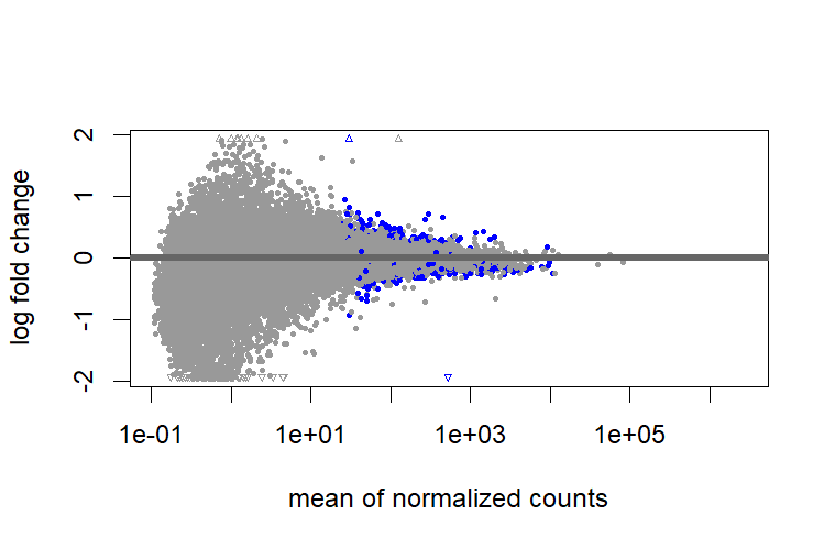
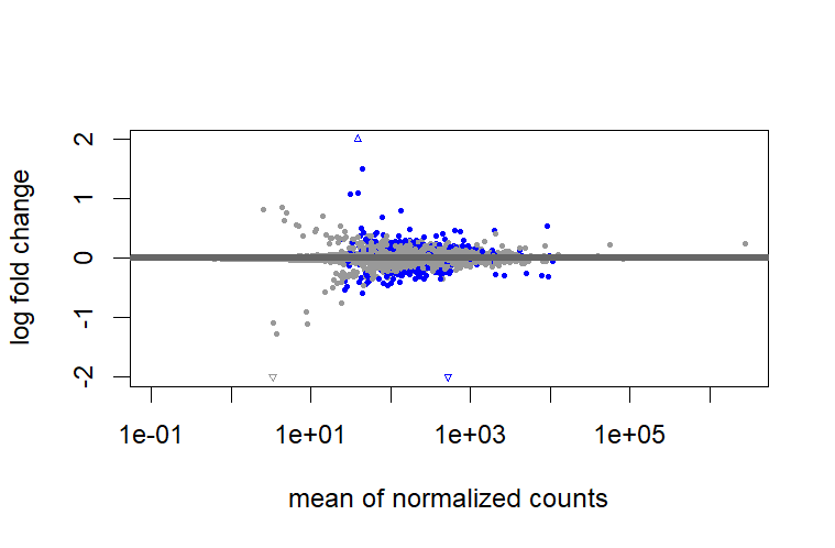
Looking at the log2FC the differences between results() and lfcShrink() are quiet different and even in opposite sign. Which one should I take into account ?

For example the top hit has a log2FC of 24.6 in results() compared to -1.27 in lcfShrink() . Differences is not very good to me. even if p-value are very low. Could someone clarify this point for me ?

enter image description here

deseq2 shrinkage • 2.8k views

ADD COMMENT • link updated 2.0 years ago by Michael Love 43k • written 4.8 years ago by Nicolas Rosewick ▴ 20

score 1 · Answer 1 · 2020-02-19

1

Entering edit mode

Michael Love 43k

@mikelove

Last seen 12 hours ago

United States

I'd recommend here 1) to use test="LRT" and results for each contrast of interest which will produce better rankings for these multiple group comparisons, or alternatively 2) to use lfcShrink with type="apeglm" or "ashr" and svalue=TRUE to rank your genes. I have seen with multiple groups and when there are these kinds of bimodal expression patterns (e.g. B in the above gene), that the Wald statistics are overly sensitive to a few samples with high counts.

ADD COMMENT • link 4.8 years ago Michael Love 43k

0

Entering edit mode

Thanks Michael.

I followed your first recommendation :

dds <- DESeqDataSetFromMatrix(countData = counts,colData = metadata,design = ~ group + gender)
dds <- estimateSizeFactors(dds)
keep <- rowSums(counts(dds, normalized=TRUE) >= 10) >= 5  # min 5 samples with 10 normalized reads
dds <- dds[keep,]
dds <- DESeq(dds)
res.wald <- results(dds,contrast=c("group","B","A"))

dds.LRT <- DESeq(dds,test="LRT",reduced = ~gender)
res.LRT <- results(dds.LRT,contrast=c("group_detail","B","A"),test="LRT")

And here is the differences in terms of adjusted p-values. LRT test seems less conservative. However some of the top hist using LRT are not significant at all in Wald test e.g. ENSG00000159176.14

Ordered by padj_LRT :

                   log2FC_wald  pvalue_wald    padj_wald log2FC_LRT    pvalue_LRT      padj_LRT
ENSG00000133392.18  -1.3243384 2.441976e-05 2.361609e-04 -1.3243384 1.109787e-116 4.487314e-112
ENSG00000198467.15  -1.5174517 5.978108e-08 1.289167e-06 -1.5174517 7.928895e-115 1.602985e-110
ENSG00000182253.15  -1.1874501 1.596151e-03 7.830475e-03 -1.1874501 4.374298e-112 5.895678e-108
ENSG00000101335.10  -1.4674044 1.328076e-06 1.908295e-05 -1.4674044 3.526412e-109 3.391887e-105
ENSG00000159176.14  -0.1537638 4.560953e-01 6.124998e-01 -0.1537638 4.194351e-109 3.391887e-105
ENSG00000149591.17  -0.5710111 1.733808e-02 5.389162e-02 -0.5710111 9.402238e-107 6.336168e-103
ENSG00000079308.19  -1.5308015 2.114945e-08 5.239932e-07 -1.5308015 8.323485e-105 4.807883e-101
ENSG00000243480.7   -6.5606656 8.145424e-24 3.293521e-20 -6.5606656 2.052341e-101  1.037305e-97
ENSG00000196924.17  -1.4946616 2.524870e-09 8.306801e-08 -1.4946616  3.642032e-96  1.636244e-92
ENSG00000172403.11  -1.2327279 1.163188e-04 8.815809e-04 -1.2327279  2.256487e-95  9.123880e-92

Here's the number of genes with padj < 0.01 for both wald and LRT test :

       sig_Wald
sig_LRT FALSE  TRUE
  FALSE 18909   593
  TRUE  12890  8042

In red : genes with padjLRT < 0.01 and padjwald > 0.01

enter image description here

I'm kind of confuse which test to use. Could you clarify which one to use and/or maybe give me some links explaining when to use either Wald or LRT ?

Thank you Nicolas

ADD REPLY • link 4.8 years ago Nicolas Rosewick ▴ 20

0

Entering edit mode

I’ve found LRT to be better in these cases of multigroup comparisons with bimodal expression vs 0’s. It is less likely to find these genes to be significant.

ADD REPLY • link 4.8 years ago Michael Love 43k

0

Entering edit mode

Hi Nicolas,

I am just confused if you want to compare the difference among 7 groups, the design should be design = ~ gender + group, right?

ADD REPLY • link 2.1 years ago Yijing • 0

0

Entering edit mode

Hi Michael,

do yo mean that if I use test = " LRT", I don't need to shrink?

But when I use test = " LRT", I found there are big differences between shrunk and unshrunk data. Why and how these differences will influence further analysis? enter image description here

However, it cannot shrink the data for comparison between two groups that are not baseline.

> res_HomHet_shrunken <- lfcShrink(dds, coef = "Genotype_Hom_vs_Het", type = "apeglm")
Error in lfcShrink(dds, coef = "Genotype_Hom_vs_Het", type = "apeglm") : 
  coef %in% resultsNamesDDS is not TRUE

Here, I have Hom, Het and WT 3 groups and WT is the baseline.

ADD REPLY • link 2.1 years ago Yijing • 0

0

Entering edit mode

It's hard to compare LRT and the posterior estimates. I'd just stick with one approach I think, maybe for you the LRT.

ADD REPLY • link 2.1 years ago Michael Love 43k

0

Entering edit mode

Sorry, could you explain more why we do not need to shrink if using LRT?

ADD REPLY • link 2.1 years ago Yijing • 0

0

Entering edit mode

LRT gives a p-value which is valid for inference of multiple coefficients. You can just focus on the coefficients from significant genes, as those typically have reliably estimated LFC.

ADD REPLY • link 2.0 years ago Michael Love 43k