Hi, I'm trying to assess differential expression in my total RNASeq data. I have several groups: Baseline, infected Pathogen1, infected pathogen 2, infected pathogen 1+2) where infected groups were sampled across 4 days. Pathogen 1+2 at 7 days has only 2 samples where the rest have 4 samples at each time (except baseline n=3). I'm planning to compare all of the groups (considering each time point from the infected groups as separate group) using a linear model to baseline.

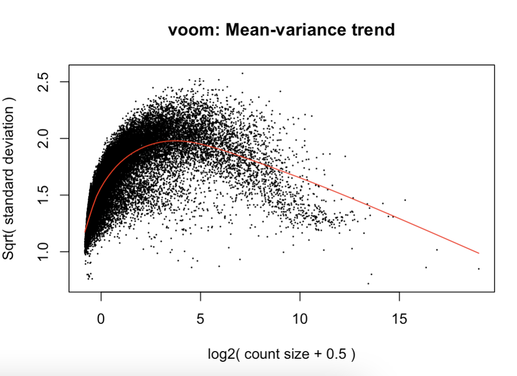
I'm concerned about the plot of mean variance trend because it looks like I have not filtered the data sufficiently- the trend resembles a normal curve (ref: https://stats.stackexchange.com/questions/160255/voom-mean- variance-trend-plot-how-to-interpret-the-plot & Law et al., 2018). I'm not sure what the best approach would be to remedy this as suggested in Law et al. if I need to filter more.

Note: Filtering based on the group with the least amount of samples (2) and for cpm considered an avg of 5 million reads per sample (range: 27k - 10 million)

#1d. Create DGElist, d1
d0 <- DGEList(mouse.counts)
head(d0)
dim(d0) #134,071 x 49

## PREPROCESSING AND NORMALIZATION  

# 2. FILTER genes that have CPM values above 2 in at least two libraries: 
keep <- rowSums(cpm(d0) > 2) >= 2
d <- d0[keep, , keep.lib.sizes=FALSE]
dim(d) #29089 genes remaining

#Calculate norm factors after filtering.
dt <- calcNormFactors(d)
dt$samples

dgex2 <- estimateCommonDisp(dt, verbose=TRUE)
degxplot2 <- plotBCV(dgex2) #BCOV 3.7

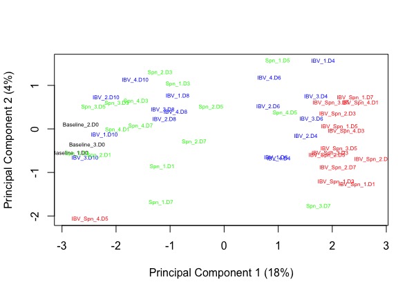
#Look at the multidimensional scaling plot
#MDS plot colored by "Group' ordering: (color, #of samples corresponding to this color), cex is the font size, pairwise comparisons 
plotMDS(dt,  col=c(rep("black",3), rep("red",4), rep("red",4), rep("red",4), rep("red",2), rep("blue",4), rep("blue",4), rep("blue",4), rep("blue",4), rep("green",4), rep("green",4), rep("green",4), rep("green",4)), cex=0.3)
#common genes for each comparison
plotMDS(dt,  col=c(rep("black",3), rep("red",4), rep("red",4), rep("red",4), rep("red",2), rep("blue",4), rep("blue",4), rep("blue",4), rep("blue",4), rep("green",4), rep("green",4), rep("green",4), rep("green",4)), cex=0.5, gene.selection = "common")

#Write the log-transformed normalized expression data (filtered data)
logcpm <- cpm(dt, prior.count=2, log=TRUE)
avelogcpm <- aveLogCPM(dt)
hist(avelogcpm)

##DESIGN MODEL MATRIX
group <- metadata1$Group #metadata table considers each tx & day as a separate group
group <- factor(group)
table(group)
Baseline.D0  IBV_Spn.D1  IBV_Spn.D3  IBV_Spn.D5  IBV_Spn.D7      IBV.D1      IBV.D3      IBV.D5 
          3           4           4           4           2           4           4           4 
     IBV.D7      Spn.D1      Spn.D3      Spn.D5      Spn.D7 
          4           4           4           4           4 
mmg <- model.matrix(~group)
ydt <- voom(dt, mmg, plot = T) #norm factors calculated on filtered data

#test model fitting
#fitting linear models with Limma 
fit <- lmFit(ydt, mmg)
head(coef(fit))
plotSA(fit)

#6b. Empirical Bayes smoothing of standard errors (shrinks standard errors that are much larger or smaller than those from other genes towards the average standard error) (see https://www.degruyter.com/doi/10.2202/1544-6115.1027)
efit <- eBayes(fit)
head(efit)
plotSA(efit)
sessionInfo( )

ydt <- voom(dt, mmg, plot = T)

You could use filterByExpr(), as recommended by Law et al (2018) and in the limma and edgeR case studies.

However, the main problem with your data seems to be the huge about of variability between replicates (BCV = 3.7), and no amount of filtering will help with that.